
Steve Randy Waldman writes the blog interfluidity. His take is usually away from the mainstream, and always interesting.
~~~
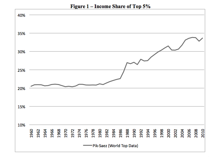
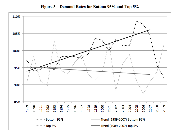
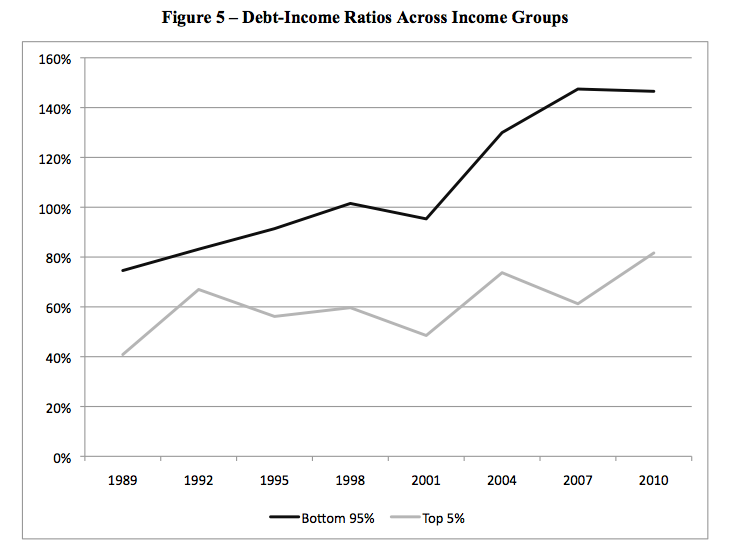
Teaser: The following graphs are from “Inequality and Household Finance During the Consumer Age“, by Barry Cynamon and Steven Fazzari. “Demand rates” are expressed as fractions of “spendable income”. There’s more on this paper at the end of the post.
I am always outclassed by my correspondents and commenters. The previous post on inequality and demand was no exception. I want to follow up on a few scattered bits of that conversation. I apologize as always for all the great writing, in comment threads and in e-mails, that I fail to respond to.
First, I want to make a methodological point. Several commenters (e.g. beowulf, JKH, Mark Sadowski) point to discrepencies between measures of income and saving used by various empirical studies and those used in national accounting statements (e.g. NIPA). In particular, there is the question of whether unspent capital gains (realized or unrealized) should count as saving. NIPA accounts quite properly do not treat capital gains as income.
But what is proper in one context is not proper in another. NIPA accounts attempt to characterize the production, consumption, and investment of real resources in the consolidated aggregate economy. A capital gain represents a revaluation of an existing resource, not a new resource, and so properly should not be treated as income.
However, when we are studying distribution, what we are after is the relative capacity of different groups to command use of production. We must divide the economy into subgroups of some sort, and analyze interrelated dynamics of those subgroups’ accounts. Capital gains don’t represent changes in aggregate production, but they do shift the relative ability of different groups to appropriate that output when they wish to. When studying the aggregate economy, capital gains should be ignored or netted-out. But when studying distribution — “who owns what” — capital gains, as well as the dissaving or borrowing that funds those gains, are a critical part of the story. Research on how the distribution of household income affects consumption absolutely should include capital gains. There are details we can argue over. Unencumbered, realized capital gains should qualify almost certainly as income. Gains from favorable appraisal of an illiquid asset probably should not. Unrealized gains from liquid or hypothecable assets (stocks, real estate) are shades of gray. There is nothing usual about shades of gray. All spheres of accounting require estimation and judgment calls. Business accountants learn very quickly that simple ideas like “revenue” and “earnings” are impossible to pin down in a universally satisfactory way.
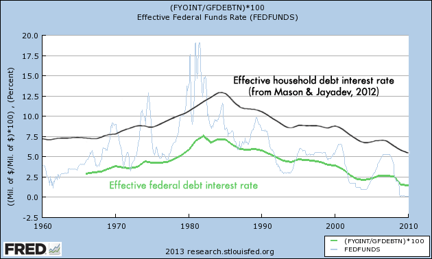
Similar issues arise in interpreting the excellent work of J.W. Mason and Arjun Jayadev on household debt dynamics, to which Mark Sadowski points in the comments. Mason and Jayadev decompose the evolution of the United States’ household sector’s debt-to-income ratio, breaking down changes into combinations of new borrowing and interest obligations (which increase debt-to-income) plus inflation and income growth (which decrease debt-to-income). It’s a wonderful, fascinating paper. If you’ve not done so already, I strongly recommend that you give it a read. It’s accessible; much of the tale is told in graphs. (A summary is available at Rortybomb, but you want to study especially Figure 7 of the original paper.)
One of Mason and Jayadev’s most interesting discoveries is that the period since the 1980s has been an “Era of Adverse Debt Dynamics”, a time during which household debt-to-income increased because of reductions in inflation, low income growth and a high effective interest rate on outstanding debt. [1] For most of the period from 1980 to 2000, the aggregate US household sector was not taking on new debt. Household sector debt-to-income deteriorated despite net paydown of imputed principal, because of adverse debt dynamics.
So, can a theory that claims borrowing by lower-income households supported demand over the same period possibly be right? Yes, it can. At any given time, some groups of people are repaying debt and others are taking it on. If, say, high income boomers are paying off their mortgages faster than low-income renters are borrowing to consume, new borrowing in aggregate will be negative even while new borrowing by poorer groups supports demand. (Remember how back at the turn of the millennium we were marveling over the “democratization of credit“?)
As always, when studying distributional questions, aggregate data is of limited use. That’s not to say that there is no information in aggregate data. It’s definitely more comfortable to tell the borrowed demand story about the 2000s, when, Mason and Jayadev show us, aggregated households were dramatically expanding their borrowing. But what we really want is research that disentagles the behavior of wealthy and nonwealthy households.
A working paper by Barry Cynamon and Steven Fazzari does just that. It tells a story quite similar to my take in the previous post, but backs that up with disaggregated data. The three graphs at the top of this post summarize the evidence, but of course you should read the whole thing. There is stuff to quibble over. But the paper is an excellent start.
I’ll end all this with an excerpt from the Cynamon and Fazzari paper that I think is very right. It addresses the question of why individuals would undermine their own solvency in ways that sustain aggregate spending:
It is difficult for standard models, most notably the life cycle model, to account for the long decline in the saving rate starting in the early 1980s. A multitude of economists propose explanations including wealth effects, permanent income hypothesis (high expected income) effect, and demographics, but along with many researchers we find those explanations unsatisfying. We argue that the decline in the saving rate can best be understood by recognizing the important role of uncertainty in household decision making and the powerful influence of the reference groups that to which those household decision makers turn for guidance. We propose that households develop an identity over time that helps them make consumption decisions by informing them about the consumption bundle that is normal.9 We define the consumption norm as the standard of consumption an individual considers normal based on his or her identity (Cynamon and Fazzari, 2008, 2012a). The household decision makers weigh two questions most heavily in making consumption and financial decisions. First, they ask “Is this something a person like me would own (durable good), consume (nondurable good), or hold (asset)?” Second, they ask “If I attempt to purchase this good or asset right now, do I have the means necessary to complete the transaction?” Increasing access to credit impacts consumption decisions by increasing the rate of positive responses to the second question directly, and also by increasing the rate of positive responses to the first question indirectly as greater access to credit among households in one’s reference group raises the consumption norm of the group. Rising income inequality also tends to exert upward pressure on consumption norms as each person is more likely to see aspects of costlier lifestyles displayed by others with more money.
People will put up with almost anything to live the sort of life their coworkers and friends, parents and children, consider “normal”. Over the last 40 years, for very many Americans, normal has grown increasingly unaffordable. And that created fantastic opportunities in finance.
[1] Mark Sadowski suggests that the stubbornly high effective interest rates reported by Mason and Jayadev are inconsistent with a claim that the secular decline in interest rates was used to goose demand. But that’s not quite right — it amounts to a confusion of average and marginal rates. At any given moment, most household sector debt was contracted some time ago. The effective interest rate faced by the household sector is an average of rates on all debt outstanding, and so lags headline “spot” interest rates. But incentives to borrow are shaped by interest rates currently available rather than rates on debt already contracted. Falling interest rates can increase individual households’ willingness to borrow much more quickly than they alter the aggregated sector’s effective rate.
In my first encounter with the Mason and Jayadev paper, I thought I saw in the stubbornly high effective rates evidence of a rotation from more-creditworthy to less creditworthy borrowers. (See comments here.) I’ve looked into that a bit more, and the evidence is not compelling: the stubbornly slow decline in household sector interest rates pretty closely mirrors the slow decline in the effective interest rate of the credit-risk-free Federal government. There’s a hint of spread expansion in the late 1990s, but nothing to persuade a skeptic.
This entry was posted on Tuesday, February 12th, 2013 at 6:08 pm EST and is filed under uncategorized. You can follow any responses to this entry through the RSS 2.0 feed. You can leave a response, or trackback from your own site.
~~~
http://www.interfluidity.com/v2/3972.html

What's been said:
Discussions found on the web: